
We are releasing three Kimi K3 draft models trained with TorchSpec:
All three models were trained in disaggregated mode using 40 GB200 GPUs. The corresponding training recipes are available in TorchSpec. This post compares the released checkpoints and describes the architecture, training, and data-pipeline improvements that made the runs practical.
| GPUs | 40 (8 training + 32 inference) |
| Max Context | 64K tokens |
| Training examples | 300K lightseekorg/kimi-mtp-dataset regenerated |
Because of resource constraints, the released DSpark checkpoint was trained for fewer epochs than DFlash2; its results are therefore not a fully matched comparison.
Benchmark results
Acceptance length
We compared the three draft checkpoints across 10 benchmarks spanning math, code, retrieval/QA, Chinese, and dialogue. All benchmarks use temperature 1.0, top_p 0.95, and maximum reasoning effort. EAGLE3 runs at draft/verify depth 3/4; DFlash2 and DSpark run at draft/verify depth 7/8.
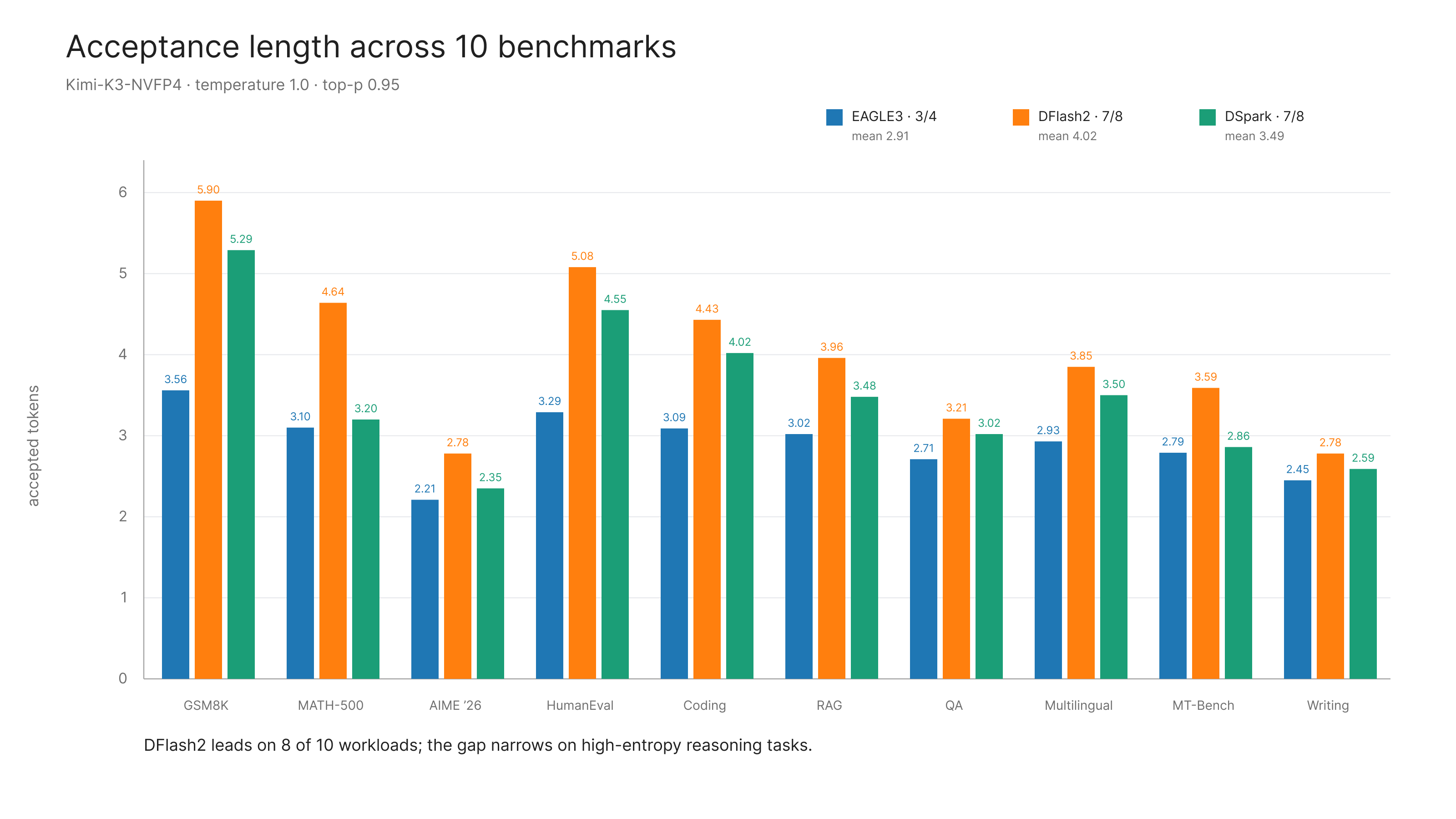
Figure 1. Acceptance length across 10 benchmarks.
End-to-end throughput
Acceptance length alone does not determine serving performance, so we also measured end-to-end throughput with each draft model integrated into the engine. We used the mixed low-, medium-, and high-entropy workloads from SPEED-Bench under the same sampling settings as above. This workload is intended to approximate the diversity of production traffic.
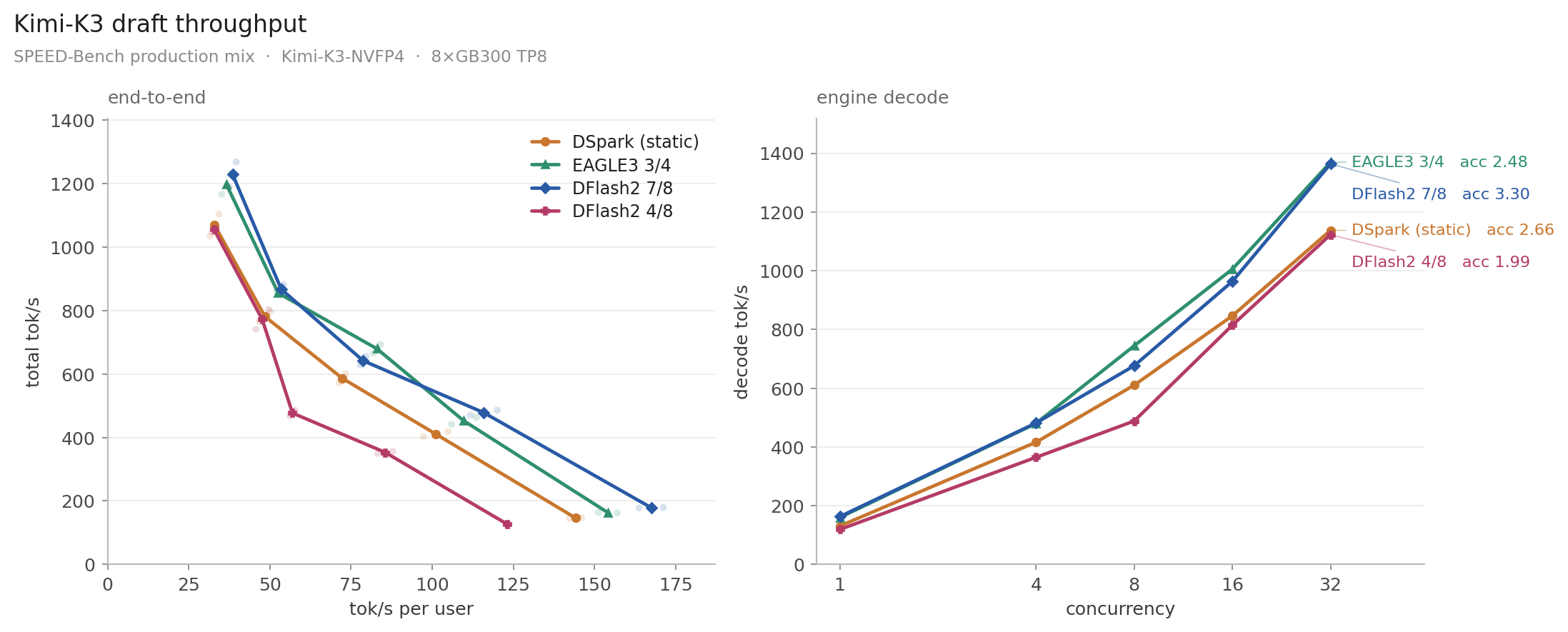
Figure 2. Kimi K3 SPEED-Bench throughput sweep.
DFlash2 outperforms EAGLE3 at lower concurrency, while the gap narrows as concurrency increases. The DSpark result is more preliminary: the released checkpoint was trained for fewer epochs, and this benchmark did not use dynamic verification, which could avoid work on low-confidence drafts. We therefore treat this sweep as a comparison of the released configurations rather than a definitive ranking of the algorithms.
DFlash2 has an advantage at lower batch sizes because it generates more draft tokens in one block, so a longer accepted prefix removes more serial target steps. Beyond a batch size of 32, however, the higher acceptance length no longer compensates for verifying the additional positions. At temperature 1.0, later positions are less likely to be accepted, and much of the extra verification work is discarded; EAGLE3's shorter 3/4 window wastes less of that tail. Two other properties of K3 make wider verification more expensive:
- K3 is a sparse MoE. Extra verify tokens scale expert FLOPs and dispatch with verify width, not just with tokens that survive rejection.
- K3 is a 3:1 hybrid of KDA and gated MLA. KDA must advance and rewind recurrent state per speculative token, which means more states and larger graph replays as draft width grows. Full-MLA models such as Kimi K2.6 can reuse compressed KV across extra query tokens, so additional verify positions have more gains from attention computation.
Draft architectures
TorchSpec now supports training both DSpark and DFlash2 draft models for Kimi K3. We validated both paths in full training runs and used them to produce the released checkpoints. The implementations are general enough to support further experiments with draft architectures tailored to different deployment constraints.
All three draft models use Multi-Latent Attention (MLA), which reduces KV-cache storage and integrates cleanly with prefill/decode disaggregation and a unified KV-cache layout. In long-context benchmarks, attention became a bottleneck for the draft models, motivating us to evaluate Sliding Window Attention (SWA) in the first four layers.
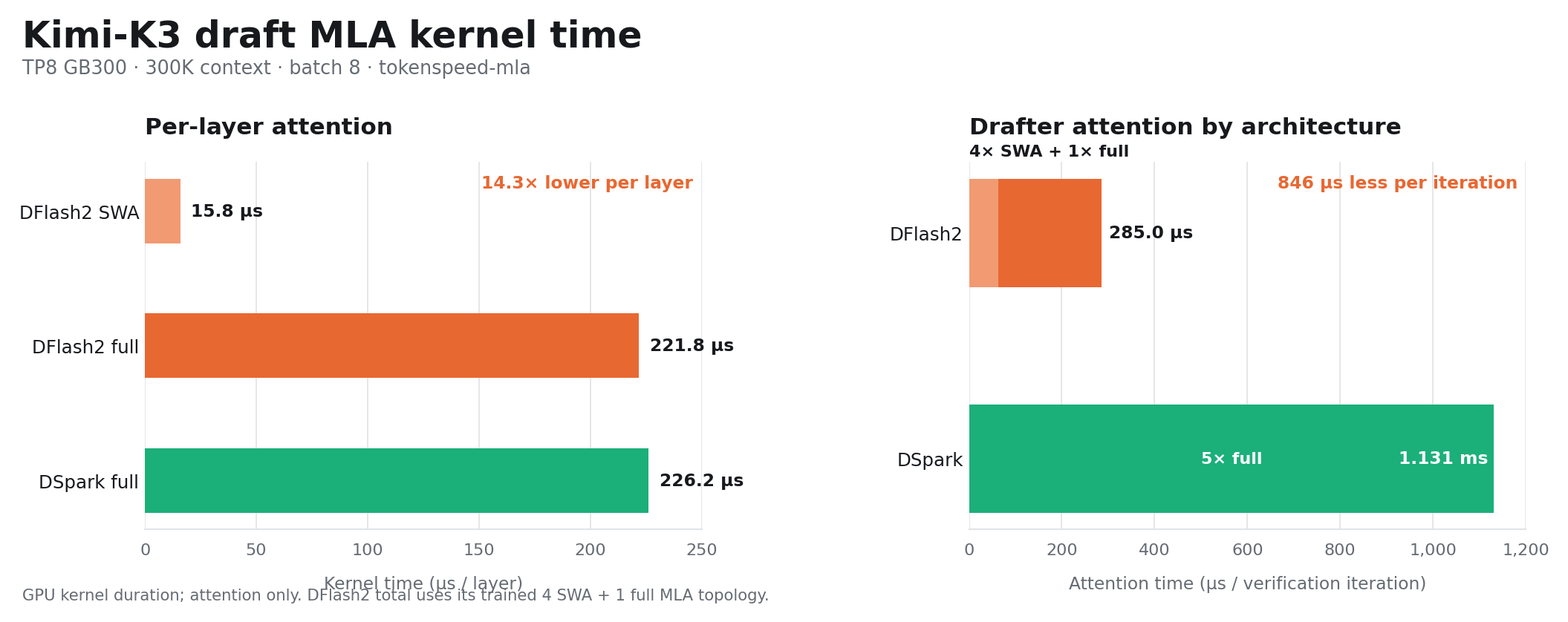
Figure 3. Draft MLA kernel-time comparison.
DFlash2 is trained with four SWA layers and one full-MLA layer; DSpark is trained with five full-MLA layers.
Training efficiency improvements
We removed bottlenecks from both the training loop and data preprocessing. On 4×GB200 with a batch size of 2, the combined training optimizations improved throughput by 2.5×.
Pipeline-parallel support
Kimi K3 does not fit on eight GB200 GPUs, so the target model must be sharded across 16 GPUs. Pipeline parallelism replaces much of the all-reduce traffic required by other sharding strategies with point-to-point hidden-state transfers at pipeline-stage boundaries. TorchSpec now supports general pipeline-parallel execution with vLLM as the inference engine. Each stage collects hidden states and writes them to Mooncake asynchronously, overlapping data movement with computation and reducing pipeline bubbles.
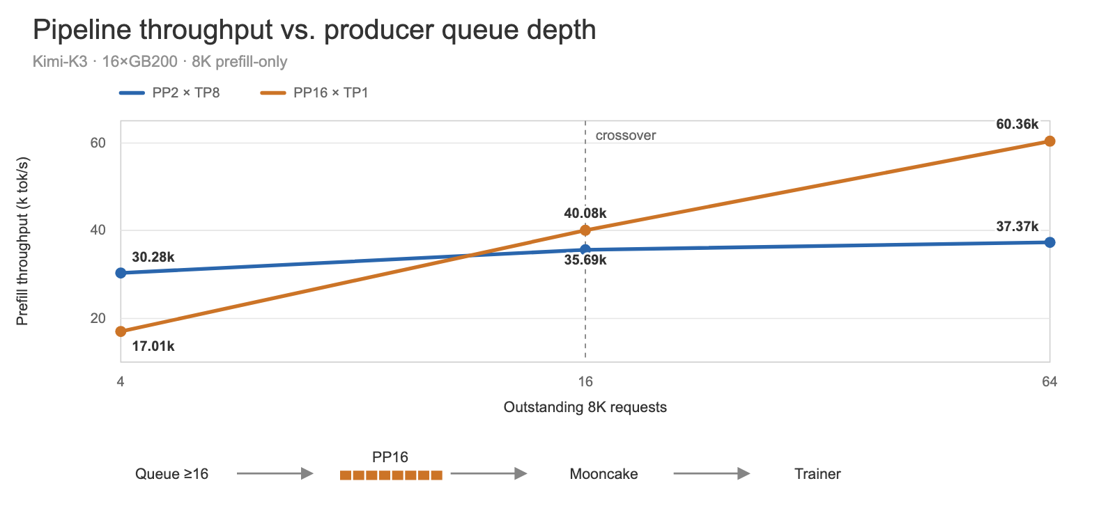
Figure 4. Pipeline-parallel prefill throughput scales with the outstanding producer queue while Mooncake decouples inference from training.
Anchored EAGLE
EAGLE-3 traditionally trains with a TTT rollout at every token. This becomes expensive in both memory and runtime for long sequences because every position receives a TTT prediction.
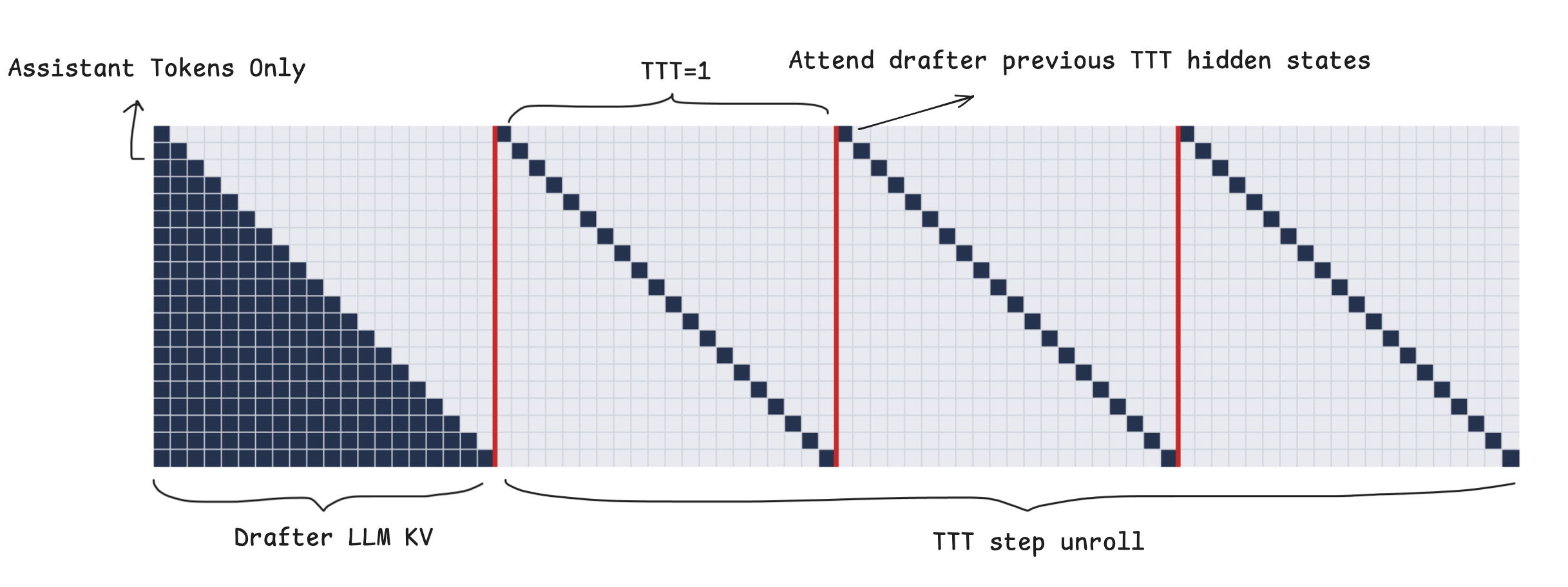
Figure 5. KV cache mask visualization for the EAGLE's TTT training.
DFlash instead samples random "anchor tokens" and predicts N-token block continuations from each anchor. A bidirectional attention mask isolates each block prediction. Because the number of anchors does not grow with sequence length, long examples do not dominate the run, making training more stable at long context.
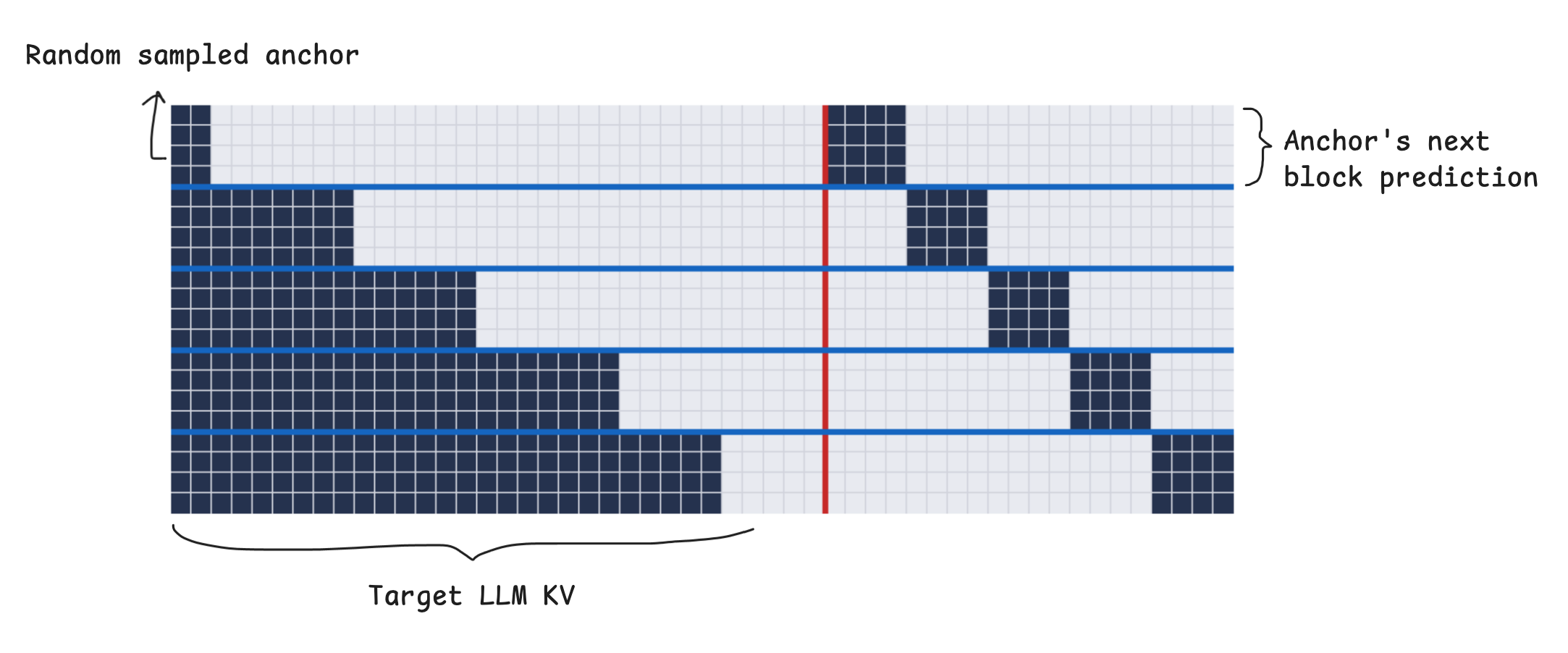
Figure 6. KV cache mask visualization for DFlash training.
We apply the same anchoring idea to EAGLE training: instead of running TTT rollout at every position, we sample anchor tokens. Unselected tokens still contribute through the KV cache, so full rollout coverage is not required to obtain a useful training signal.
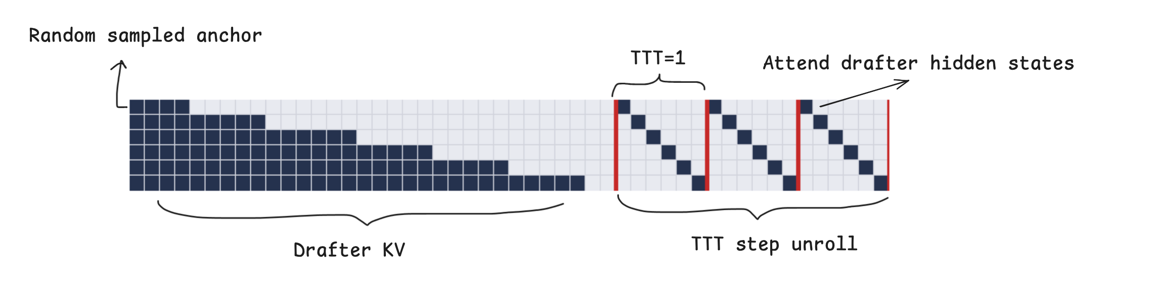
Figure 7. KV cache mask visualization for anchored EAGLE training.
This samples a comparable number of positions from inputs of different lengths. Anchoring lets the same drafter capacity absorb more varied data while substantially reducing unnecessary attention computation and HBM usage.
| seq | dense TTT | anchored SDPA | speedup |
|---|---|---|---|
| 4096 | 2.89 / 0.92 | 1.21 / 0.43 | 2.4x |
| 16384 | 34.27 / 4.20 | 2.17 / 1.60 | 15.8x |
| 32768 | 127.48 / 7.91 | 4.02 / 3.17 | 31.7x |
Table 1. Attention-computation speedup from anchored EAGLE for the MLA drafter.
Grouping sequences by length
Speculative decoding training can scale by increasing the number of data-parallel workers or by increasing the batch size. Larger batches work well because training is largely memory-bandwidth-bound by the EAGLE TTT calculations. However, naive batch-size scaling does not produce a linear speedup.
The main source of wasted work was padding. Sequences of different lengths must be padded to a common shape within a batch and across workers, causing the model to process tokens that do not contribute to training.
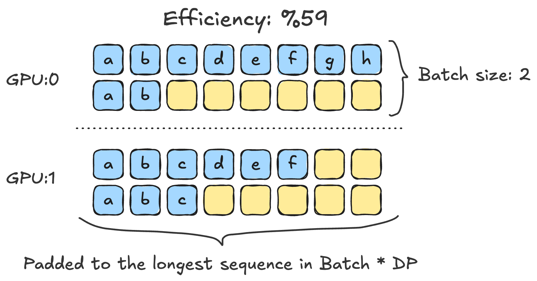
Figure 8. Initial training sequences. Yellow squares represent wasted padding.
We now sort sequences by length and group similarly sized sequences into the same batches. This reduces padding and increases the amount of useful work performed by each training step.
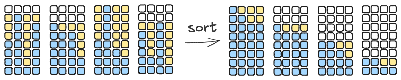
Figure 9. Length-sorted sequences. Yellow squares are remaining padding; white squares are padding that can be skipped.
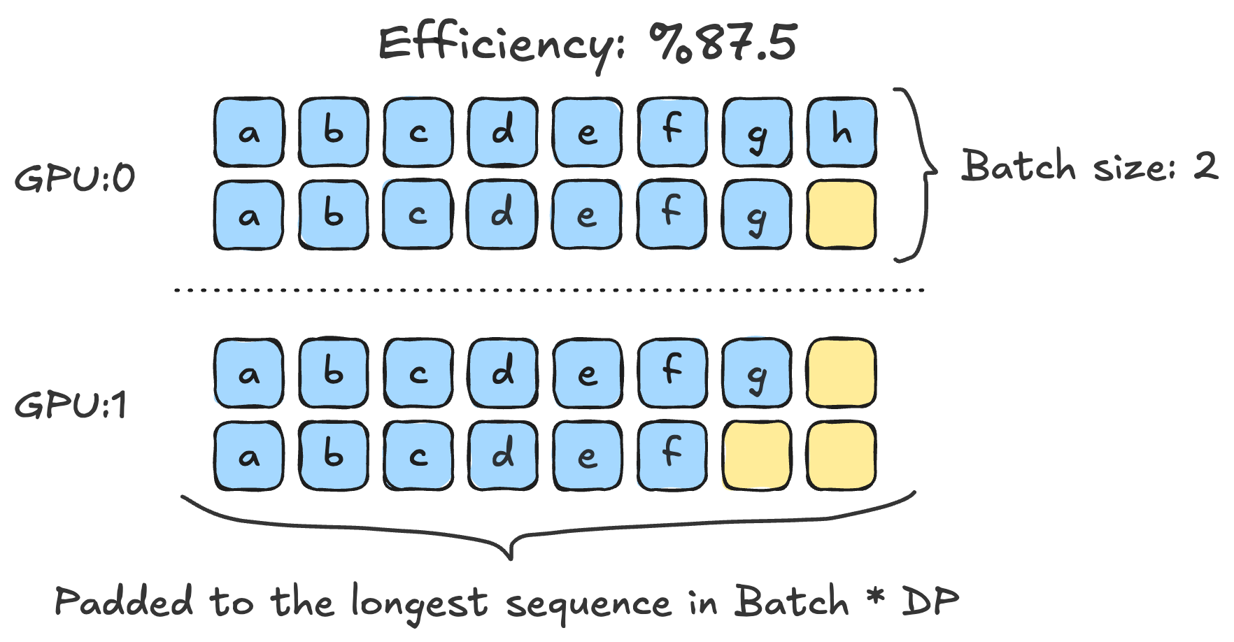
Figure 10. Training batches after length-based grouping.
Removing CPU synchronization
Calls to .item() on the main thread forced the CPU to wait for pending GPU operations. Some values, such as training metrics, eventually need to reach the CPU, but they do not need to block the current step. We therefore defer metric reporting by one step.
We also switched to the fused Adam optimizer and replaced Python loops with torch._foreach_ operations. Together, these changes keep the CPU from unnecessarily stalling GPU execution.
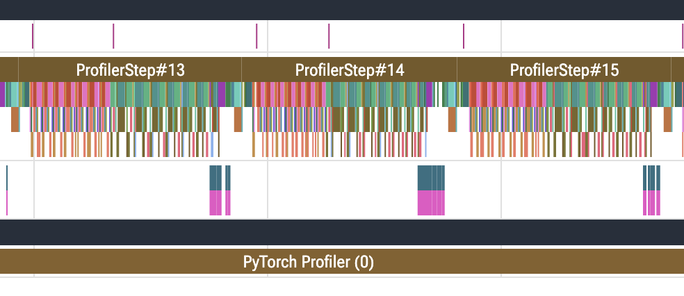
Figure 11. Torch Profiler trace before removing main-thread synchronization.
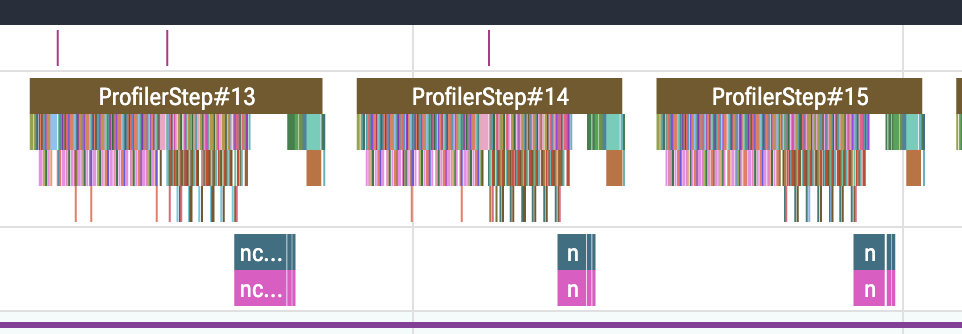
Figure 12. Torch Profiler trace after removing main-thread synchronization.
4.5x faster preprocessing
Before training begins, TorchSpec converts raw conversations into token IDs. The result is cached, but preprocessing remains on the critical path for every new dataset. At the scale of one million conversations, two multiprocessing behaviors made this stage unnecessarily expensive.
Workers returned PyTorch tensors to the parent process. PyTorch transfers tensors between processes through shared memory, with each tensor consuming a file descriptor. This works well for a small number of large tensors, but one million small results can exhaust the parent's file descriptors. Returning NumPy arrays as bytes and converting them with torch.from_numpy reduced result collection from 498 seconds to 23 seconds.
Creating the worker pool before loading the dataset also lets each worker inherit an empty list and receive only its assigned inputs through the work queue. This reduced tokenization time for one million rows from 1,436 seconds to 319 seconds.
Offline training for experiments
TorchSpec now also supports an offline training workflow. Normally, the target model and draft trainer run concurrently: the target generates hidden states, sends them through Mooncake, and the trainer consumes them. Whichever side is slower throttles the other, and both workloads compete for available GPUs.
Offline training separates the workflow into two phases. The target model first materializes hidden states to disk. The draft model then trains against those files without keeping the target model online. This is useful when GPUs are constrained, when repeatedly experimenting on a fixed dataset, or when inference and training need different cluster layouts.
# Phase 1: materialize hidden states on the inference GPUs
python -m torchspec.offline.generate \
    --config configs/your_config.yaml \
    --output ./data/hidden-states

# Phase 2: configure the trainer to consume the materialized data
# inference:
#   inference_engine_type: offline
#   offline:
#     data_path: ./data/hidden-states
#     num_engines: 4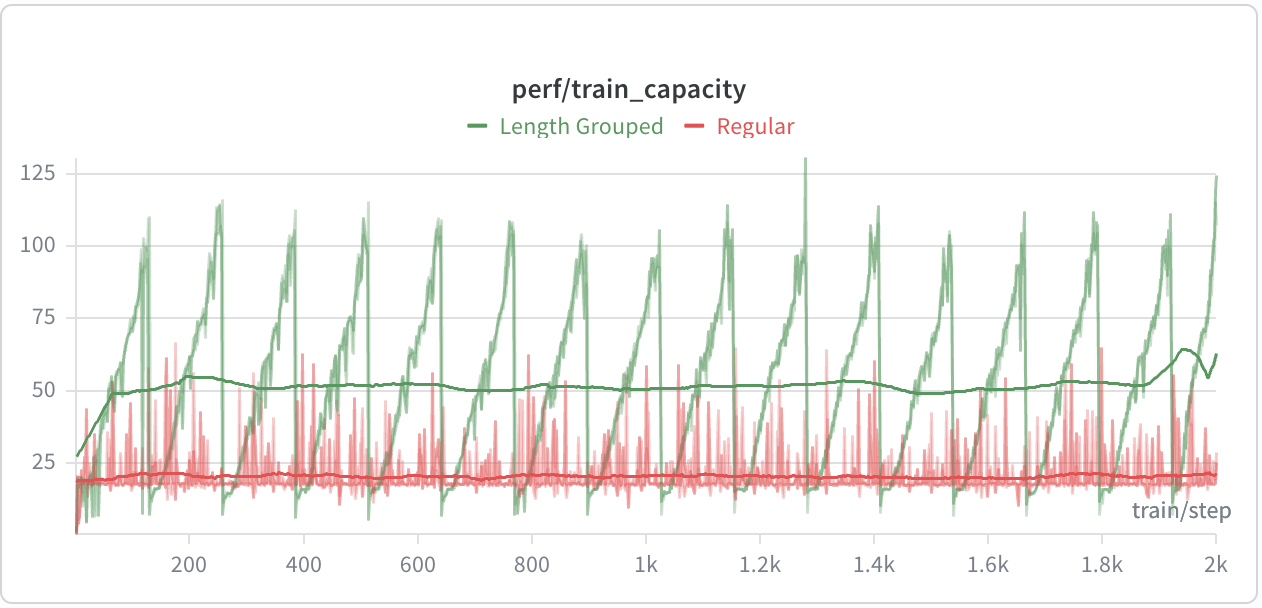
Figure 13. Final training-speed improvement on 4×GB200 with batch size 2.
Reproducible builds and nightly CI
Model support remains difficult to use when it depends on a collection of local patches. Each user must identify compatible revisions, apply the same changes, build the environment, and repeat correctness checks. Small differences in any of those steps make failures difficult to reproduce.
We now publish Docker images containing the required vLLM patches and run nightly CI over the TorchSpec training workflow. The nightly job verifies that training completes and that convergence remains within the expected range.
Users can therefore start from a prebuilt environment instead of rebuilding the patch stack locally. This reduces setup time, catches compatibility regressions earlier, and gives developers and users a shared baseline when debugging.
Takeaways and next steps
The results show that draft-model quality cannot be reduced to acceptance length alone. On Kimi K3, the best serving configuration depends on concurrency, verification width, and the cost of advancing the model's sparse MoE and hybrid KDA/MLA state. DFlash2 leads at lower concurrency in our released configuration, while EAGLE3 becomes more competitive as concurrency increases.
The training-system work is equally important to that comparison. Pipeline-parallel hidden-state generation, anchored EAGLE training, length-aware batching, deferred CPU synchronization, and faster preprocessing collectively make long-context draft training more efficient and easier to reproduce. Offline training and prebuilt Docker images then turn those improvements into a reusable workflow rather than a one-off run.
These checkpoints and recipes are intended as reproducible starting points, not a final ranking of speculative decoding methods. A matched follow-up should train each model under comparable budgets, enable dynamic verification for DSpark, and repeat the serving sweep as engine support evolves.
References
- Yuhui Li, Fangyun Wei, Chao Zhang, and Hongyang Zhang. EAGLE-3: Scaling up Inference Acceleration of Large Language Models via Training-Time Test. NeurIPS 2025.
- Jian Chen, Yesheng Liang, and Zhijian Liu. DFlash: Block Diffusion for Flash Speculative Decoding. ICML 2026.
- Inco AI. DFlash 2: Keep Drafting Parallel. 2026.
- Xin Cheng et al. DSpark: Confidence-Scheduled Speculative Decoding with Semi-Autoregressive Generation. 2026.